
You are reading the full technical report — every method, every honest limit, every interactive demo. For the short commercial overview, start here ←.
Measuring on photographs — the method.
Sub-millimeter answers from the photos you were shooting anyway — perspective included. Others deliver pictures; a PhotoRobot sweep delivers pictures that answer questions. Every image leaving the studio doubles as a measurement record: any bolt, radius or spacing can be dimensioned later, by anyone, without touching the part again.
A global vehicle-benchmarking provider digitises 200–500 technical parts per shift on PhotoRobot lines using exactly this method.
The problem — why this page exists
PhotoRobot customers are very often suppliers of technical goods: spare parts for machines and vehicles, electronic components, fittings, tooling. When their buyers ask for the real dimensions of a part, the reflex answer today is a 3D model — photogrammetry from a large set of frames, or lately a Gaussian splat. Both work, and both carry the same costs: glossy, translucent or untextured surfaces — the everyday reality of technical parts — break or degrade the reconstruction, and even on top-end PhotoRobot lines a successful model costs minutes of post-production per part plus a denser shot set. Every one of those minutes comes straight out of studio throughput.
So the question this page answers: what if measuring worked on the basic shot set, with zero post-production? There is a whole ladder of methods — from laying a printed measuring strip next to the part and reading dimensions against it, up to full 3D computation from two or three calibrated frames. The chapters below walk that ladder with interactive demos at every rung, and at the end you verify the accuracy yourself, on a real cast gearbox. The pay-off is practical: ship your customers photographs with the key dimensions already booked, or let them measure whatever they need to check, directly on your website — so they buy right the first time. Your customers will appreciate it, and so will whoever runs your returns desk.
Where this sits — and why it costs no studio time
A word before the numbers. If you need the whole part, exactly, the answer is a parametric 3D model — and a PhotoRobot line can deliver that too, by classical photogrammetry, within photogrammetry’s well-known limits: glossy and transparent parts resist reconstruction, and while the remedies exist, they slow a production line down. What this page presents is different. It measures on a single photograph — or on a positionally defined set the robot captures automatically — at no capture cost — on photographs you were taking anyway: the sweep takes about twenty seconds, everything is online in under a minute, and the measurements land with an accuracy that tends to surprise people. That trade — no extra capture, no reconstruction queue, exact numbers where the method’s rules hold — is what the rest of this article describes.
The outputs come from three types of measuring method, each with its own accuracy and its own distortions — naive, plane and 3D, in the demo below. PhotoRobot_controls supports all three natively — to our knowledge the only mass-deployed product-hosting system with deep-zoom that does — and the demo lets you understand each one and try it in practice.
Compose your measuring strip
The measuring strip in the scene below is not a fixed prop — it is the customer’s own artwork, and three variables build it: the logo, the color, and the scale style. Any logo format a browser can draw works: PNG, JPG, SVG, WebP, GIF or BMP. Pick a scale style below — the PhotoRobot checkerboard reading 1 / 10 / 100 mm at three zoom levels, or a classic tick ruler — and the finished assembly prints into the measuring scene, color and all. Try it now: click the mark on the left to swap in your own logo and set both colors to your brand — the strip you compose here is the very strip used in the interactive demos and examples further down the page, so the rest of your read happens in your own livery.
Try the mistake first
Below is a cube with 100 mm edges, rotated 30° on a PhotoRobot table, with a calibrated checkerboard strip — fine stripes at the cap, checker cells, color-vs-tint blocks; logo left, units right — the same artwork reads at three scales, and its length is a variable too: 50 mm reading down to 0.5 mm for screws, 100 as the default, 200 and 500 for a car door — along the front edge. The cube is drawn to machine-drawing convention: visible edges solid, hidden edges dashed. Every edge of the cube is exactly as long as every other — although the lines drawing them are visibly not. The two through-holes are ⌀20 mm, drilled on the top face's centerline, 25 mm either side of center — 50 mm apart, hole to hole. The drawing says so the way a drawing should: centerlines dash-dot, the hidden bore walls and the exit on the bottom face dashed. Perspective still renders the two identical mouths as ovals of different sizes. Click two points to measure — a loupe with a crosshair rides your cursor for precise picks. Three measuring engines sit above the drawing as tabs, and they are a ladder: Naive is what a plain pixel ruler does — right only at table level, shown so you can feel the mistake. Plane is single-view metrology: one photograph, exact in any plane you name — the everyday workhorse for flat features. 3D is stereo triangulation on two frames of the sweep: click the same feature in both and get a true point in space — no plane named, no strip needed; use it for anything oblique. Start naive on a top edge and climb the ladder. The guidance is not decoration: on a spare-parts marketplace a mis-measured part is a mis-ordered part and a return — walking every user to an exact number is precisely the cost this system exists to eliminate.
Naive measuring
What a plain pixel ruler does: pixels × the strip’s table-level scale, applied everywhere. Correct on the table, visibly wrong on anything raised — this is the mistake the whole page is about, and the window below lets you commit it deliberately.
Keyboard: ⇧ Shift+click chains dimensions · Ctrl/⌘+click (or ⇧ back to the start point) closes the loop — enclosed area, and on a raised plane the prism volume beneath it · Alt+click removes the last point · Esc cancels a half-made pick, twice clears the measurement. Mouse & touch: drag the scene sideways to rotate it (each window separately in the 3D tab), drag up/down to change the camera elevation, mouse wheel or trackpad/touch pinch to zoom — snapped points survive a view change by reprojection.
Plane measuring
Single-view metrology: one photograph, but you first name the plane you measure in, and the mathematics rescales the reference to it. Exact for flat features — top edges, the top-face diagonal, even floor→top through space with a plane per point.
Keyboard: ⇧ Shift+click chains dimensions · Ctrl/⌘+click (or ⇧ back to the start point) closes the loop — enclosed area, and on a raised plane the prism volume beneath it · Alt+click removes the last point · Esc cancels a half-made pick, twice clears the measurement. Mouse & touch: drag the scene sideways to rotate it (each window separately in the 3D tab), drag up/down to change the camera elevation, mouse wheel or trackpad/touch pinch to zoom — snapped points survive a view change by reprojection.
3D measuring
Stereo triangulation: click the same feature on two calibrated frames and the rays meet in space — true 3D, no plane to name, no strip needed. One honest note: the split window is a classroom device, here to make the two-frame idea visible. Real measuring helps itself more elegantly, as you will see on the gearbox below — a slight automatic turn of the part (the angle is configurable in the administration) fetches the confirming frame, and no screen ever splits.
Keyboard: ⇧ Shift+click chains dimensions · Ctrl/⌘+click (or ⇧ back to the start point) closes the loop — enclosed area, and on a raised plane the prism volume beneath it · Alt+click removes the last point · Esc cancels a half-made pick, twice clears the measurement. Mouse & touch: drag the scene sideways to rotate it (each window separately in the 3D tab), drag up/down to change the camera elevation, mouse wheel or trackpad/touch pinch to zoom — snapped points survive a view change by reprojection.
Check yourself — three measurements, three known answers
The cube gives you ground truth for free — every answer below is knowable in advance, so your clicks grade themselves. Work down the list; it climbs from a line to a solid. If a number refuses to match, look first at which engine and target are active:
- An edge. Target Cube top · +100 mm, click two adjacent top
corners — any of the four edges, however long its line looks.
expected: 100.0 mm - The face diagonal. Same target, click two opposite corners of the top face.
expected: 141.4 mm — exactly 100·√2 - The body diagonal. Target 3D · floor→top, click a
bottom corner first, then the top corner diagonally opposite across the whole cube.
expected: 173.2 mm — exactly 100·√3, measured through space - The top face — one for the showmen. Target Cube top · +100 mm,
⇧ Shift+click the four top corners and close the loop (Ctrl/⌘, or ⇧ back to the start).
expected: 4 × 100.0 mm · area 10 000 mm² · prism volume below: exactly one litre - A side face. Target 3D · floor→top, chain the four corners of a
vertical face — two on the floor, two on the top.
expected: perimeter 400.0 mm · area 10 000 mm² — and no volume: a vertical sheet has no column of space beneath it - The whole solid. Switch to 3D measuring and collect three
mutually perpendicular faces (close each with Ctrl/⌘, or by returning to its first point).
expected: box volume √(A₁·A₂·A₃) = exactly one litre — the cube knew it all along
For a spare check, either hole mouth measures 20.0 mm across, front or back — however different their ovals look; a single click on a hole center dimensions it whole. Then switch to Naive measuring and watch a top edge grow by 6.7 % — millimeters it never had. Turn on the Checkerboard overlay to see why: fifty-millimeter squares, identical in the world, visibly unequal on screen.
The cube is the classroom. The next iteration of this page runs the same canvas over a photographed technical part — same clicks, same mathematics, real bolts and fillets — as soon as the studio assets land.
A word on the units: engineering drawings use decimal inches, but a US shop floor reads a tape measure in binary fractions — halves, quarters, eighths, sixteenths. The switcher does the conversion the way a machinist would: 88.9 mm ÷ 25.4 = 3.5 in, shown as 3 1/2 in; a sixteenth is ~1.6 mm, which is exactly why fractional readings are for the shop floor and decimal ones for the drawing office.
You have just measured on a calibration cube — a body built to be friendly. The same two ideas run below on a real cast gearbox ↓
Two photographs, two methods
Before we go on: from here, the measuring strip retires. It earns its keep in two roles. As a physical strip laid into the picture, it is the reference of last resort for the case the mathematics cannot cover — PhotoRobot supplies these to customers made to order, with their logo and in their colors, exactly as you composed one above. And as a virtual strip, calibrated to the customer’s specific optical setup, it can be printed into any frame after the fact, with no physical handling at all. But the charm of strong mathematics is that the photographs usually need neither: the chapters that follow measure without a strip in sight — and for the cross-check, the manufacturer’s data sheets of the demonstration gearbox are further down this page, so you can hold the measured numbers against the maker’s own. Leaving the strip out will prove to be the right call.
The geometry below is here for the curious (and for the record). If maths is not your idea of a good afternoon, skip straight to the clickable demos — they carry the whole point without a single formula.
You have just used both ideas without a single formula — which is the point: the demo sells the result, the theory below explains it for the engineers who ask. The whole story fits into two pictures of the same part. The first could come from any camera. The second comes from a PhotoRobot sweep — and the difference between them is not the image, it is what can be measured from it.
Why the strip must stretch
A pinhole camera scales everything by its distance from the optical center. A feature at height h is closer to the camera than the table, so the strip that calibrates the table is too short for it — by an exactly computable amount:
S = 300 · 965 / 726.5 = 398.49 mm — the strip must appear 32.8 % longer in the raised plane.
That handles features facing the camera. Inside the picture itself, perspective adds a second distortion: parallel edges converge towards vanishing points, so the same millimeter is a different number of pixels at each end of the part. The correction is a chain of four plane triangles anchored to the two vanishing points U₁, U₂ of the scene:
- Raise the measuring plane above the base from point C — law of cosines gives the
slant side and its angle.
c = √(a² + b² − 2ab·cos γ) = 1295.15 px · β = 78.49°
- Project that height into vanishing point U₂ — a second cosine-rule triangle
across the top edge.
c = 8009.74 px · β = 8.32°
- Intersect with the rays of U₁ — law of sines recovers the side that carries
the plane's height in image space.
a = c · sin α / sin γ = 1587.36 px
- Close the chain: the corrected strip width in the raised plane.
b = 2544.49 px — versus 2062.69 px at table level
None of this needs depth sensors, stereo rigs or AI guesswork. This is single-view metrology: metric measurement from one perspective image, built on one printed strip, one calibrated robotic scene, and geometry that has worked since the Renaissance — applied carefully.
Beyond flat planes — measuring through space
A photograph records directions, not depths: every pixel is a ray. That is why a single image can measure only where the plane of each point is known — and why the vanishing points matter, because they recover the full directional grid of the scene, so any nameable plane works: horizontal, vertical or inclined. And once each point carries its own plane, the distance between them can be taken through space itself.
Try it above, in Plane measuring: select 3D · floor→top, click a bottom corner of the cube and then the opposite top corner. The reading is 173.2 mm — the space diagonal, exactly 100·√3. A vertical-face diagonal, bottom corner to the top corner above it, reads 141.4 mm — the same 100·√2 as on the top face, now measured through two different planes at once.
One honest limit remains, and it is fundamental: a single photograph cannot measure two points whose planes nobody can name. In production that limit falls too — the robot photographs every part from a full calibrated sweep, and a detail seen from two known angles is triangulated in full 3D, no plane assumption needed. One photo measures in planes; the robotic set measures space. And you can try exactly that above: the 3D measuring tab shows two frames of the sweep side by side — click the same corner in both and the rays meet in a real 3D point, no plane button anywhere. Both windows rotate through the sweep’s calibrated stops, and that rotation is not a gimmick: it solves the hidden-point problem (occlusion). A feature visible from one angle may sit behind the part from another — and stereo triangulation needs the point seen in both frames. When a corner hides, you turn either window to a stop where it shows; because every stop of the sweep is calibrated, any pair of viewpoints measures equally well. The only rule is parallax: views closer than 20° apart gray out, because near-parallel rays cannot fix depth — the demo refuses the pair instead of measuring it badly.
Proof, not promise
During the pilot we measured a raised feature physically and compared three numbers: the naive prediction from table-level scale (922.8 px), the perspective-corrected prediction (1070.1 px), and the physical measurement (1069.9 px). The naive reading was off by 15.9 %. The corrected model landed within 0.02 %.*
The third method plays by different rules, and the difference is worth naming. Plane measuring leans on the printed strip and on knowing which plane you are in — its error budget is calibration plus how well the plane assumption holds. Triangulation needs no strip and no plane: two calibrated frames carry everything, and its error budget is the calibration of the two camera positions plus how precisely the same feature is picked in both. It even audits itself — the two rays should meet, and the ray gap the demo reports is that audit: near zero when both clicks hit the same corner, obviously wrong when they do not. Flat features go to the plane method for speed; oblique geometry, free-form edges and anything between planes go to triangulation.
The rules that make it work
None of the above is magic, and it must not be sold as magic. The accuracy holds because the scene obeys a short list of rules — they are not fine print, they are the method:
- Calibrate the optical assembly first. Camera position, optical center
and lens distortion are mapped on a known target before the first measurement. Every
number on this page inherits its accuracy from that step.
recalibrate after any change — a lens swap, a knock, a remount
- Fixed focal length. A prime lens by preference; if a zoom must be used, it is locked in position and never touched — a millimeter of zoom silently rewrites the scale of everything.
- Fixed focus and aperture. Refocusing shifts the optical center (focus breathing). Focus and aperture are set during calibration and stay put.
- Stabilisation off. Optical stabilisation moves lens elements by design; the pinhole model assumes they do not move.
- Defined, repeatable angles. The robot shoots from calibrated positions. A hand-held photo has no known geometry — which is exactly why the ordinary photograph needs a reference strip in the scene and the robotic one does not.
- A rigid scene. Reference and part sit on the same rigid table. Anything that flexes between calibration and exposure is measured as flex.
- Measure in the calibrated frame. Viewers may scale images freely for display — every click is mapped back to the calibrated pixel grid before a single millimeter is computed, so the on-screen size never touches the result.
- Verify continuously. A reference object stays measurable in the scene; when its numbers drift, the system flags itself for recalibration before anyone trusts a reading again.
Which angles to shoot — heights live near the horizon
A sweep that photographs beautifully and a sweep that measures well are not quite the same sweep, and the difference is not the number of frames — it is where they are taken from. This is measured, not asserted: refitting a real part with one elevation ring left out each time shows which ring was carrying which dimension.
| Rings used | Height read back | Fit residual |
|---|---|---|
| −30° / 10° / 30° | 10.44 mm | 1.42 px |
| −30° / 30° — the near-horizon ring removed | 0.79 mm | 9.18 px |
| 10° / 30° | 12.54 mm | 0.62 px |
| −30° / 10° | 11.72 mm | 0.62 px |
Take away the ring near the horizon and the height collapses to a tenth of itself. Take away a high ring and almost nothing happens. The reason is geometric rather than photographic: near the horizon a millimetre of part height moves the outline by a large fraction of a millimetre on the sensor, while from overhead it barely moves it at all. Diameters behave the opposite way. Relative sensitivity, with each column scaled to its own best case:
| Camera elevation | Signal for HEIGHT | Signal for DIAMETER |
|---|---|---|
| 0° (dead level) | 100 % | 45 % |
| 5° | 58 % | 49 % |
| 10° | 59 % | 59 % |
| 20° | 24 % | 95 % |
| 30° | 16 % | 76 % |
| 45° | 14 % | 100 % |
| 60° | 7 % | 80 % |
| 80° (near plan view) | 2 % | 81 % |
Dead level is not required. Photographers routinely lift the camera five or ten degrees to hide the near rim of a plate or a dish, and that habit costs very little: at 10° roughly six tenths of the height signal survives, which is plenty. It is the jump from 20° to 30° that hurts — by then three quarters of it is gone, and past 45° a height is being inferred rather than seen.
- One ring near the horizon — anywhere from 0° to about 15°. Heights,
thicknesses and steps come from here, and from nowhere else.
5–10° is fine — shoot what looks right
- One ring around 30° — it ties heights to diameters and gives the parallax that turns two views into a 3D point.
- One ring high, or straight down — diameters, concentricity, bores at their full size.
- A third ring is the referee. Two rings can always be made to agree;
only a third can say that they do not. On the part above the three rings disagree by about
a millimetre, and that disagreement is the honest measure of what the sweep can promise.
two views agree by construction — three views agree, or confess
- Rotation steps are cheap and, for a turned part, nearly free of information — the silhouette of a disc does not change as it turns. Twenty-four steps are plenty there; spend the extra frames on a part with features, where rotation resolves what hides behind what.
- No number of angles buys scale. A hundred views still yield shape only.
Millimetres come from a known length in the scene, or from a rig whose geometry is known.
this is the one thing a better sweep cannot fix
A word on lenses — why perspective is a resource
CAD systems let you switch perspective off and draw in axonometry; a camera never can — but it can choose how much perspective to have. Try the LENS control above: it performs a dolly zoom, scaling focal length and camera distance together so the framing holds while the perspective changes. At 24 mm-eq the cube shouts perspective — the naive error is huge, and precisely because of that the single-view method has a strong signal: the vanishing points sit close, the strip-stretch correction has something to grip. At 200 mm-eq the image compresses towards axonometry — flattering, calm, and nearly useless for single-view metrology: the vanishing points recede towards infinity, the correction runs on a whisper of signal, and small pixel errors magnify into millimeters. Wide lenses bring the opposite tax — barrel distortion that must be calibrated out. The studio sweet spot is around 85 mm-eq: proportions that sell, perspective that still measures. And this is one more quiet argument for the sweep: stereo triangulation does not care about the focal length — its depth comes from the baseline between calibrated viewpoints, so the telephoto look that flatters the product costs the two-frame method nothing.
Dimensioned spins — three ways to serve a measurement
Everything above is the exploration mode: a person asks the photograph a question and clicks the answer out of it. Production adds two more ways to serve the same mathematics. In the provider-prepared mode, recognition runs server-side after the sweep: interesting features — hole centers by sub-pixel ellipse fit, edges, corners — are detected, measured once, verified by the operator before publishing, and the dimensions then travel with the product: the customer opens a spin photograph with the key measurements already drawn in space, and nobody had to touch the part. And the combined serving pairs the two — the prepared dimensions answer the common questions, the measuring cursor answers the uncommon ones. (Not to be confused with the hybrid view in the measuring block — that name belongs to the detection ink drawn over the photograph.) A spare-parts listing where the spin itself shows the bolt circle, the bore and the mounting height — and still lets the buyer measure the one dimension the seller did not think of — is the level this system aims at. Both new modes are live above: the Prepared dims overlay draws the provider-prepared dimensions into the scene — edge, height, hole pitch and a ⌀ — reprojecting through every rotation while your own cursor measures on top; and the real β switch in the 3D tab swaps the cube for the actual photographed gearbox sweep, where a provisional calibration and the ray-gap audit make the measuring experiment honest rather than staged.
At production scale
The line photographs each part from 12 standardised robotic angles, barcode-driven — and the measurement itself is purely optical: the photos and the calibrated geometry are all it needs. Where certified block dimensions are part of the workflow, an optional Cubiscan 325 station can run alongside — though in our pilots the optical numbers have tended to be the tighter of the two, and a gauge has hard limits on object size that a turntable does not: anything the robot can rotate — packaging included, up to genuinely large goods — measures the same way. Add a system-connected digital scale (weight captured automatically, no keyboard and no human error) and the pair — certified weighing plus high-precision optical dimensions — covers what dimensioning stations are bought for, with one difference: the photos keep answering questions forever. Measurement of any detail, after the fact — a bolt spacing, a fillet radius, an embossed rib — at 200–500 parts per shift, without ever retrieving the part from the warehouse.
Measure the real part
The cube above is the classroom; this is the exam. The same measuring canvas can swap the cube for a real photographed gearbox — an (M)RT 40A worm unit, captured by a PhotoRobot sweep in 72 frames: 24 stops of 15° at three elevations — and the lowest ring is photographed from below, through the glass table, solved as its own calibration chain with the refraction absorbed, so even the underside measures. The calibration is no longer an estimate: this very sweep was shot in the same session as a serialised calibration cube, and the block runs on the chain solved from it — camera, orbit and absolute millimeters included (the chapter below tells that story). So put it to the test: the hollow output bore should read Ø19.0 mm — the catalog ground truth — with no pinning at all. The opening image has already shown you the squared-off mounting flange: four clamping holes 90° apart on a Ø 100 pitch circle, the square reading 70.7 mm a side — 100/√2, so the geometry checks itself. Now hunt the catalog sheet below: axis height 71, body width 84, flange spigot Ø95. One warning before you search: this unit’s output flange is machined square to fit the robot fixture, so the catalog’s Ø 115 bolt circle and Ø 140 flange outline are not on the photographed piece — do not hunt for what the milling machine took away. Every pick is free-hand (no model to magnetize to), the epipolar line guides your confirming click, and the ray gap reports how honestly your two picks named the same feature. This is the whole method, on a real part, in your hands — right here: the live sweep takes your measurements, the re-set data sheet just below holds the answers, and once the operator verifies a set of dimensions they appear in blue with a ✓, travelling with the product.
Three ways to measure. Click any two points and read their distance — that alone answers most questions. The same free clicking builds an arc: three points return its radius, with the expected error stated. Or switch the view to edges / hybrid and let the magnet snap your cursor to the pre-detected shapes — rims, centers and straight edges book their dimensions in one or two clicks. The magnet follows the ink: it switches on with the detected lines and rests in the plain photo view, where there is nothing to snap to.
 Settings
measure
Settings
measure
Readout
View
Measuring aids
Detection layerthe pen the magnet reads
Enclosing box
Measuring strip
Calibration & export
Settings themselves are not remembered — only your work, and only in this browser.
Tools
M magnet to entities · G magnet to the grid — both can be on, an identity always wins
⌥ drag slides the grid inside its plane (the part stays put) · ⌥⇧ drag turns it · ⌥ double-click puts it back on the part’s centre, square
⇧ click a cube face — or the grid row’s ⇓ ⇑ ⇐ to push a plane along its own normal, ∡ to tilt it — the quick way to put a plane where you measure
the grid-plane block under the navigation EDITS the plane: its name opens the list, ↺↻ turns the lattice, ⇓⇑ pushes the plane along its own normal, ∡ tilts it, ⟲ puts it all back, ⇱ moves it onto a point you click
. / , finer or coarser snap — 1 → ½ → ¼ → a tenth of the grid cell (at a 1 mm cell that is 0.1 mm)
V look straight at the active plane — the CAD ‘normal to’ move, on the plane’s own normal
D draw a sketch on the plane — point / line / arc / trace, all exact 3D; a sketched line is an edge for the ─ and ∠ tools, so an angle gets a real vertex. The sketch can be hidden and the dimensions stay.
N new plane from three points — then the grid lies in it, and one click in that plane is an exact point (dimensions at a click each)
K construction lines — a click lights a grid line; two lit lines crossing make an exact point you can measure from
R radius from three points
C centre + circumference
Esc drop the tool
⌫ delete the selected one
View
P photo
H hybrid
E edges — the detection layer
F zoom to fit
arrows step the view
X Y Z axis plane · again = far side
⇧ click a cube face lays the measuring grid on that plane, without moving the view
What the marks mean
recognised — verified across many frames
your own pick
derived — box, hidden edge, bridged circle
measurable edge or slot — click it
centre lines and the axis of revolution
⊕ exact centre — clickable
⚠ doubt — the value stands, the status line says why
Engineering tools
L edge tool — two edges: parallel = distance; the same edge twice = its length
A angle of two edges
⇥ cycles the contours under the loupe — and where the layer has nothing, it looks again on the spot
space (hold) guides the second point: horizontal, vertical or a part axis
Editing
click a dimension or its pill selects and zooms
drag a pill moves the pill · ⇧ drag moves the whole dimension (extension lines follow) · ⌥ drag walks the anchor around a circle · double-click snaps it back
⇧ click chains · Ctrl/⌘ click closes a loop → area
Alt+click deletes any of yours
Ctrl/⌘ Z puts a deleted dimension — or a deleted plane — back (20 steps)
Reading the layer
colour groups a shared plane
dashed circle = bridged from neighbouring frames — click its centre
solid stroke = seen in this very frame
teal stadium = a slot: one click books width and centre spacing
⌀ pill = a verified identity, R pill = a three-point fit
Drag turns · wheel zooms · double-click zooms to a point · ⇧ drag pans. Nothing else to learn.
Keeping a dimension straight. A hole can sit square in the photograph while your two picks do not — the line ends up a few degrees off and the dimension, though numerically right, looks hand-drawn. Hold space after the first point: guides appear through it — screen horizontal, screen vertical and the three axes of the part itself (the edges of the enclosing box, projected into this view). The cursor rides the nearest one, lit in orange, with a dot where the second click will land. Release the key and you are back to free-hand. The same applies to the confirm click in the neighbouring frame, so a dimension stays straight through the whole two-view procedure. And once a dimension is booked, its label can be dragged anywhere — the leader line follows and keeps its dot on the geometry — which is what you want before a screenshot goes into a report; a double-click on the label snaps it back to automatic placement.
A word on short-arc radii. Determining an arc from three points on a short segment is the one task where this method's usual tenths-of-a-millimeter accuracy is not enough: for a shallow arc, R ≈ c²/8s, so a tenth of a millimeter in the sagitta moves the computed radius by whole millimeters or more. The tool computes and shows this ± with every radius, and flags ill-conditioned readings with ⚠ — treat those seriously: verify by another procedure, pick the three points further apart along the arc, or use the pre-recognised geometry on the object (the blue identities), whose cross-frame voting is an order more accurate. A wrong radius sent downstream is a returned part or a mis-made counterpart.
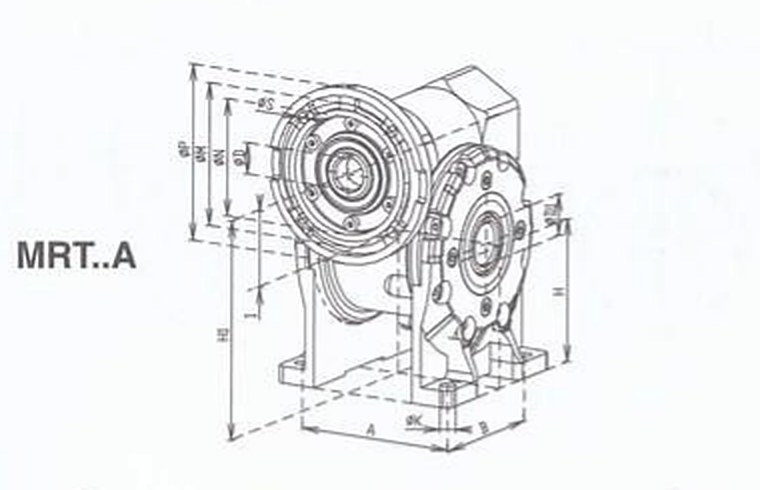
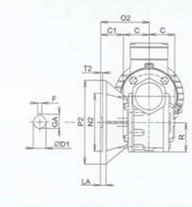
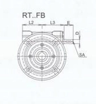
| Letter | Value (mm) | What it is |
|---|---|---|
| D1 H7 | Ø 19.0 | hollow output bore — the known dimension that pins the scale. Both ends are heavily chamfered, so the true Ø 19 edge hides between two larger rings — but the detector holds it. |
| H | 71 | shaft axis height above the feet |
| H1 | 111 | overall height |
| A | 84 | body width across the feet |
| G | 70 | housing width at the output |
| N2 H7 | Ø 95 | output flange spigot |
| M2 | Ø 115 | output flange bolt circle |
| P2 | Ø 140 | output flange outer diameter |
| D k6 | Ø 11 | input shaft diameter |
📖 The operator’s manual — every control, explained for the curious
Views. photo is the frame as shot; edges is the detection ink the magnet works from; hybrid lays that ink over the photograph — maps-style — and doubles as the quality lens: when a number surprises you, hybrid shows you why. The magnet follows the ink: on with edges/hybrid, resting in photo view. Pin your preferred view as this device’s default in ⚙.
Picking. Hover and the loupe magnifies; the card beside it names what is lit and what a click will do. Click a rim to book that circle’s ⌀ in one click (cross-frame identity, witnesses, plane depth or an admitted single-view guess — in that order of strength). Click a center to take an exact 3D point; Tab cycles overlapping candidates; a dashed guide leads to the center of the lit circle. Free clicks anywhere else triangulate through a small automatic confirm turn (size in ⚙) — Esc cancels and returns the view, zoom and pan exactly where you were.
Chains, loops, areas. After a dimension lands, ⇧-click chains the next point from the last endpoint — a bolt square is four clicks. Return to the first point and the loop closes itself: enclosed area, and for a horizontal loop the prism volume above the table. Ctrl/⌘ closes on demand; the ⚙ switch loop → area turns the behavior off.
Radius. ◠ mode takes three points along an arc and returns R with its expected error stated — a shallow arc is honest about being a poor witness. Known exact centers skip the confirm turn entirely; a click on an arc near a known center sketches the full circle from center + point.
Editing a finished dimension. Point the crosshair at it — label, line or ring — and it lights up; click selects. Then: ✕ deletes (⌫/Del too), the decimals dropdown overrides precision for that one dimension, ⌒ seat (offered only when both anchors sit near a machined plane, and only when there is something to fix) projects them onto it and reports old → new, double-click renames (“M8”), and a ⌀ dimension’s center becomes a magnet point — measure a pitch straight from it. Click elsewhere to deselect; an idle Esc never deletes.
Boxes and the strip. ⚙ can draw the table box (what a dimensioning gauge returns) and the part-axes box (the minimum cuboid in the part’s own coordinate system) — both from the visual hull of 48 silhouettes, both in the JSON export. The virtual strip glues your composed artwork to the table: it turns with the part, hides behind it on the far side, and measures true — two clicks across a 10 mm checker read 10.0.
Phone. First tap aims (loupe above the finger), a second tap nearby picks; drag turns, pinch zooms; on-canvas pills stand in for Esc and ⌫.
Try these — five minutes to conviction
A few guided runs that show the range. One: switch the view to edges, find the input-flange face and measure the spacing of its four corner holes — hover the first center, click, then ⇧-click the remaining centers: four clicks, four pitches, and the square should read close to 70.7 mm a side. Two: click the rim of any flange hole — one click, one diameter, witnesses and all. Three: switch to ◠ radius and place three points along a casting fillet — the radius arrives with its expected error stated, which is the honest part. Four: hunt the hollow output bore and compare your reading against the catalog’s Ø19.0. When a number surprises you, the hybrid view shows you why — the detection ink draws over the photograph and the disagreement is visible to the eye.
Calibration that travels with the machine
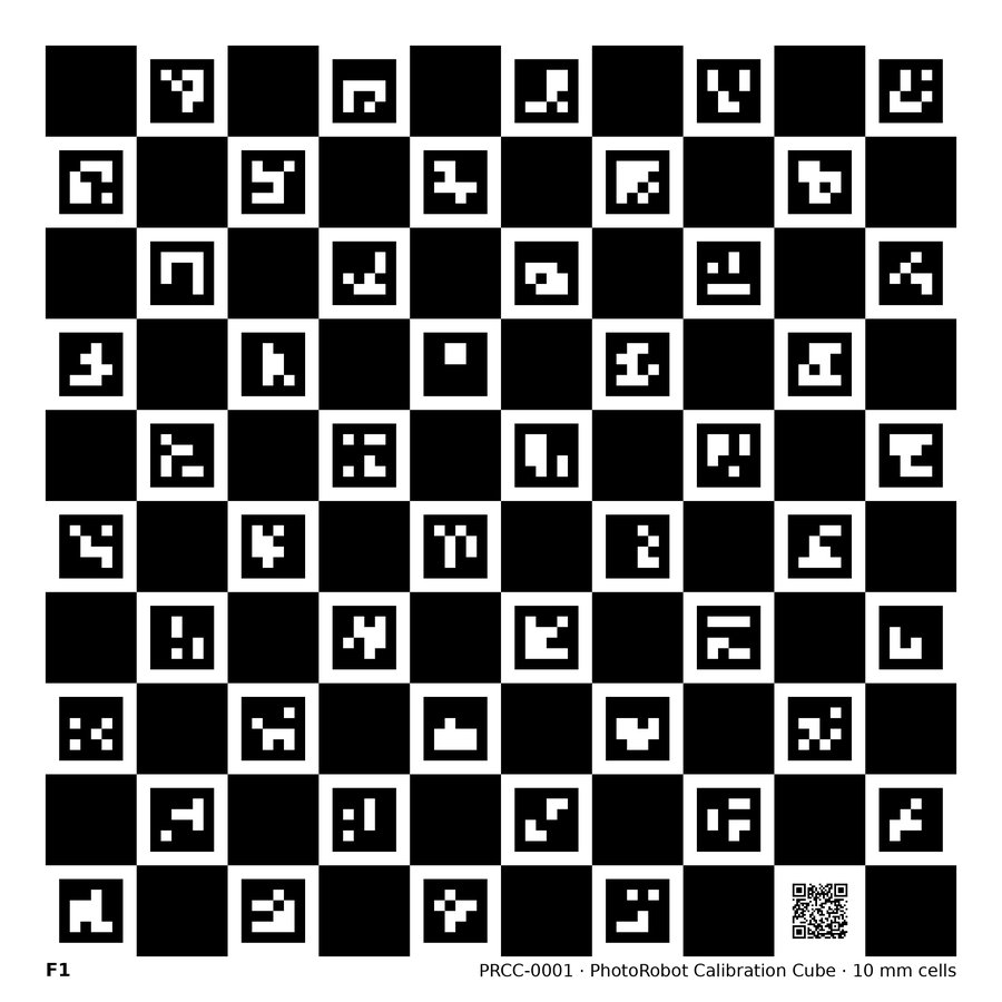
The measuring block above runs on the first production chain — solved from cube PRCC-0001, photographed on the same turntable minutes before the gearbox. This is how it works in production: every measuring rig gets a serialised calibration cube — six machine-readable grid faces, each carrying a unique block of coded markers, so any photograph that sees a patch of any face knows exactly which face it is looking at and where. Photograph the cube once on your turntable and the solver returns the complete calibration chain: the camera’s focal length and principal point, the orbit geometry, the mutual poses of all six faces (assembly precision is deliberately irrelevant — the cube surveys itself), and, because the grid pitch is a known, caliper-verified number, absolute millimeters. No manual pinning, nothing to type.
The chain belongs to the workstation, not the account. One company often shoots on several rigs — a large turntable for machinery, table-top units for parts — and each has its own optics and geometry. Each therefore has its own chain; every photo set records which chain it was born under, and the viewer loads the right numbers automatically. Recalibration adds a new chain version; nothing is overwritten, and history stays auditable. For customers with several sites this is the quiet superpower: calibration follows the machine wherever the account grows.
And one more consequence worth reading twice: if your production setup has not changed, measuring can be switched on for photos you took months ago. Photograph the cube once today, and the chain applies to every earlier sweep from the same rig — an entire archive becomes measurable retroactively. We recommend a spot-check of known dimensions across the portfolio, and the ray-gap audit keeps every individual measurement honest either way.
Each face also carries a QR code: scanning it opens the cube’s own page with its serial and a downloadable replacement print sheet. The cube is an instrument and a licence in one — every chain names the serial it was calibrated from.
Where the gauge stops — and this keeps going
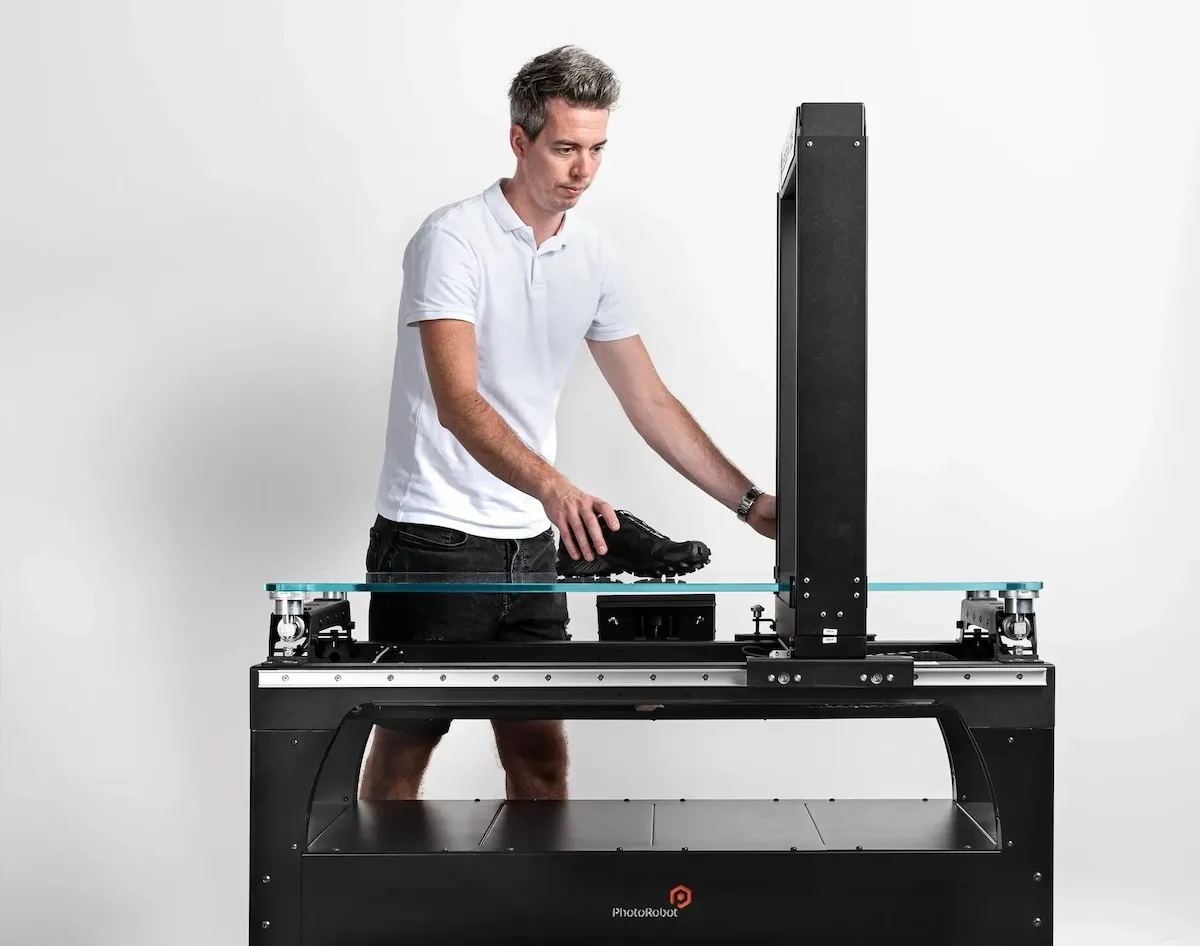
A word of respect first: Cubiscan is an excellent instrument. We have supplied these gauges to our customers for many years, and in production logistics they do exactly what they promise. But every gauge has a frame it cannot leave. Its working volume is fixed — above a certain size the part simply does not fit. And it measures the object in its resting pose: the base rectangle hugs the footprint tightly at any angle (lay a shoe diagonally and the CubiScan draws the tight rectangle around it, not around the machine axes) — but the height stays vertical and the pose stays whatever gravity chose. A part that leans on its own castings — like our gearbox — gets a box with the lean baked in.
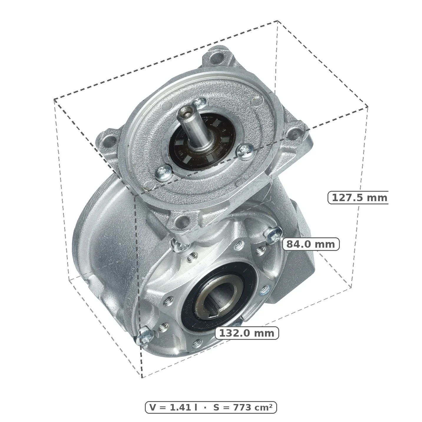
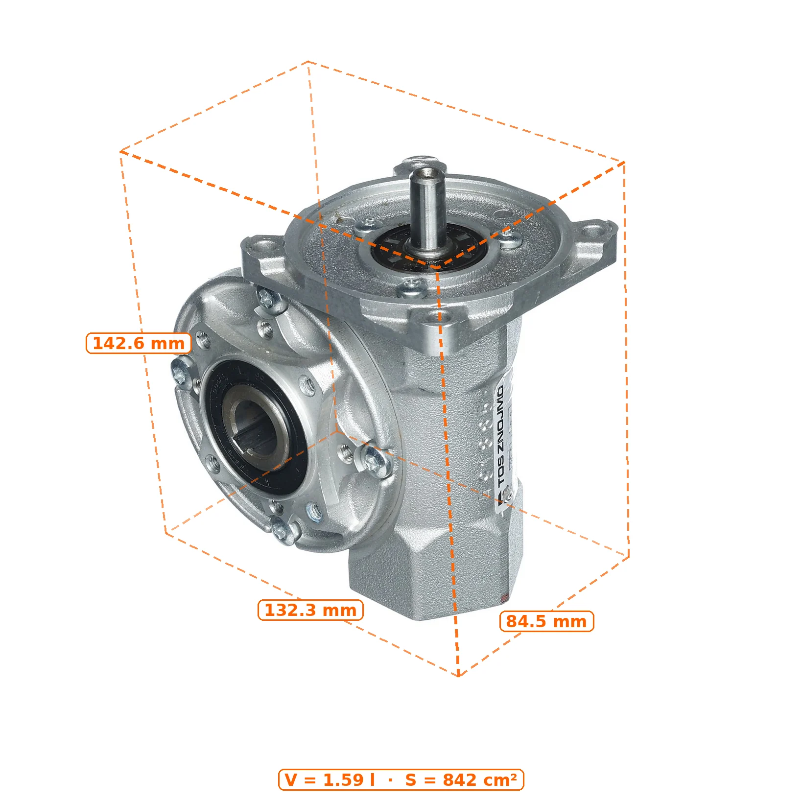
The software alternative on this page inherits neither limit — and it returns not one box but three, because three different people ask the question. The resting-pose cuboid is gauge parity: upright, its footprint rectangle minimised over rotations — exactly what a dimensioning station would print (132.0 × 84.0 × 127.5 mm here, carved from the visual hull of 48 calibrated silhouettes — the 84.0 lands on the catalog’s 84, with a millimeter of humility owed to the hull’s resolution). The true minimum cuboid is the logistics number: the smallest box the part fits in over all orientations — what decides cartons and pallet counts. A gauge cannot know it, because it only ever sees the part as it happened to stand; we search every orientation (for this unit the minimum coincides with as-it-sits — in general it need not). And the part-axes box goes where a gauge cannot. This gearbox leans a full 23.5° on the table — a gauge bakes that slouch into its numbers. Our box is built the way a machinist would clamp the part: from its datum features — the machined input-flange face (the plane of the four holes measured throughout this page) gives one axis, the bolt-square edge in that plane gives the second, and the box follows the part, not the table: 84.5 × 132.3 × 142.6 mm in the part’s own frame. The 84.5 lands on the catalog’s body width; the 142.6 runs from the input-shaft tip to the base along the flange normal — numbers a drawing would recognise, from a part that happens to be lying askew: usually the largest of the three boxes, and the one an engineer actually wanted. One more asymmetry worth saying out loud: behind every one of these numbers stand the photographs and the calibrated geometry — a gauge that fails mid-shift takes its numbers with it; here the record already holds everything, and any dimension can be re-asked years later. Add a system-connected digital scale and the pair covers the whole dimensioning-station brief — with photographs that keep answering questions forever, and every number drawn on the product itself.
Where the bar sits in numbers — the dimensioner’s published accuracy across its model range, and how this method compares at four object sizes — is set out below the price on the overview page →
What it costs
Earlier we said the measuring rides on photographs you were taking anyway — that stays true: no extra capture, no post-production, no reconstruction queue. What is priced is the service on top of them. Measuring is not part of the standard PhotoRobot_controls tariff. It is an add-on priced at €50 per month per 1 000 products hosted on PhotoRobot hosting — products, not photographs: a product’s whole sweep counts once. At full package utilisation that is 5 cents per product per month, or €0.60 per product per year — for a listing where every dimension is answerable forever.
Set against what it buys, the number is small. A buyer who can measure the part before ordering is a buyer who trusts the listing — and a buyer who ordered the right part is a return that never happened. Nowhere does this cut deeper than in spare parts: new technical components, where a flange pitch or a shaft diameter decides fit, and used parts — a dismantler’s yard where no two items are alike and no datasheet exists. One prevented return pays the measuring add-on for that product for decades; the trust it builds into every other listing comes free.
* Accuracy figures are from the pilot's validation measurement. A full repeated-measurement series is part of every production deployment — quoted tolerances are established per scene, per camera and per part class before go-live.